CS221 Artificial Intelligence - Reflex

Reflex Based Models

Reflex agent : 1. 从环境中获取输入 : 2. 通过预测器，预测输出 : 3. 输出结果

非线性

Quadratic predictors : 二次预测器

Quadratic clasifiers : 二次分类器 : Decision boundary - 一个圆

Piecewise constant predictors : 分段常数预测器

Predictors with periodicity structure : 周期性结构预测器

Linear predictors

feature template : 特征模板 : group of features all computed in a similar way : e.g. 字符串 以 .com,.cn 结尾

• dense feature
• sparse feature
  • 大量 0

Linear classifier

$$\ f_w(x)= sign(s(x,w)) = \begin{cases} +1 & \text{if} \space w \cdot \phi(x) > 0 \\ -1 & \text{if} \space w \cdot \phi(x) < 0 \\ ? & \text{if} \space w \cdot \phi(x) = 0 \end{cases}$$

Margin

• larger values are better

$$m(x,y,w) = s(x,w) \times y$$

Linear regression

$$f_w(x) = s(x,w) = w \cdot \phi(x)$$

Residual

amount by which the prediction $f_w(x)$ overshoots the target $y$

$$r(x,y,w) = f_w(x) - y = s(x,w) - y$$

Loss minimization

Loss function : 损失函数 : $Loss(x,y,w)$ : weights $w$, output $y$, input $x$.

Classification case : 分类问题

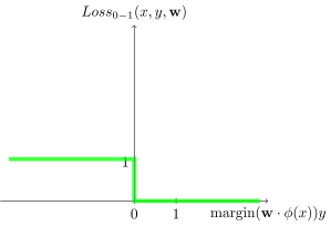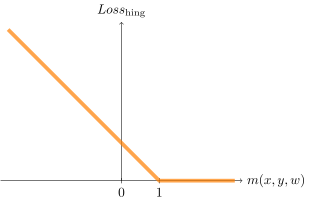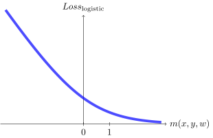Regression case

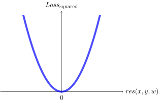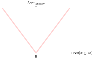Zero-one loss

$$\begin{alignat*}{2} \text{Loss}_{0-1}(x,y,\text{w}) &= 1[f_\text{w}(x) \ne y] \\ &= 1[ \underbrace{ (\text{w} \cdot \phi(x)) y }_{\text{margin}} \le 0 ] \end{alignat*}$$

Logistic regression

$$\textrm{Loos}_\text{logistic}(x,y,w) = \text{log}(1+e^{−m(x,y,w)})$$

Loss minimization framework

$$\textrm{TrainLoss}(w)=\frac{1}{|\mathcal{D}_{\textrm{train}}|}\sum_{(x,y)\in\mathcal{D}_{\textrm{train}}}\textrm{Loss}(x,y,w)$$

group DRO : Group distributionally robust optimization

$$\textrm{TrainLoos}_\text{max}(w) = \underset{g}{\text{max}} \textrm{TrainLoos}_g(w)$$ $$\nabla\textrm{TrainLoos}_\text{max}(\mathbf{w}) = \nabla \textrm{TrainLoos}_{\text{g}^\text{*}} (\mathbf{w}) \\ \text{where } g^\text{*}=\underset{g}{\text{argmax}} \text{TrainLoss}_g(\mathbf{w})$$

Non-linear predictors

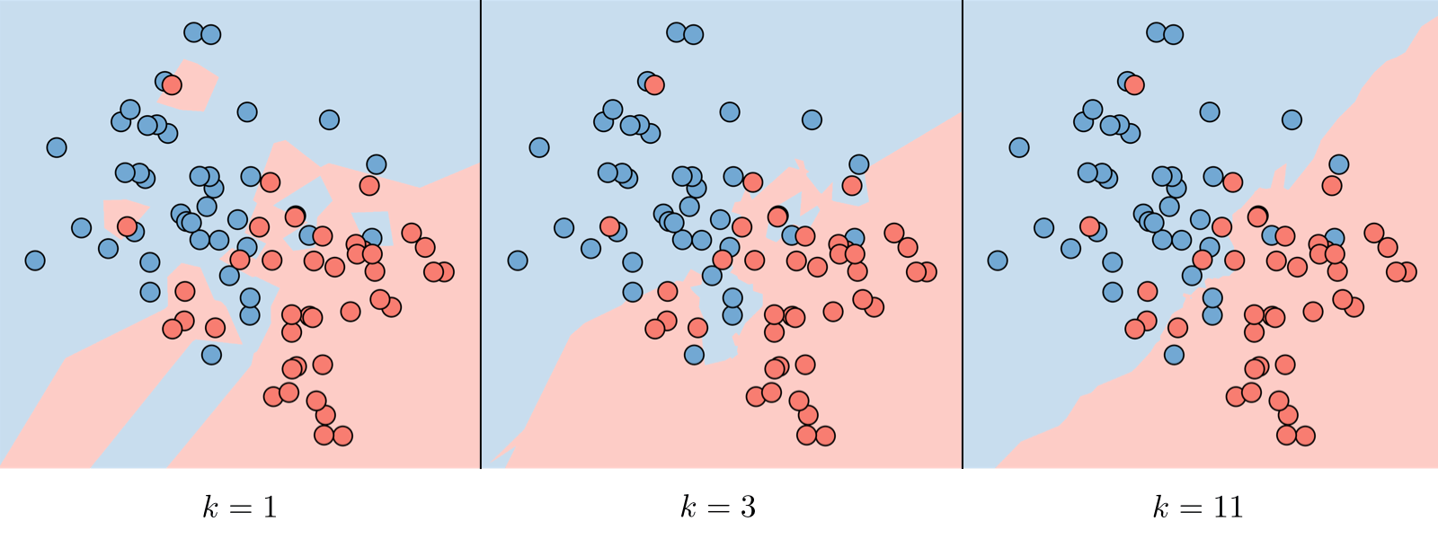
$k$-nearest neighbors : KNN : $k$相邻 : 用于分类、回归

• $k$
  • 与 bias 成正比
  • 与 variance 成反比

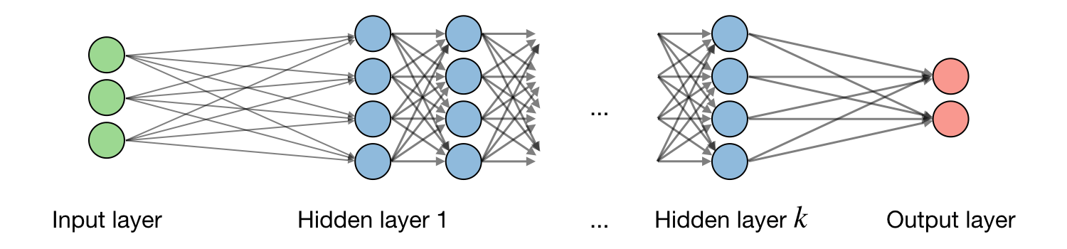
Neural networks : 神经网络

$$z_j^{[i]}={w_j^{[i]}}^Tx+b_j^{[i]}$$

• w - weight
• b - bias
• x - input
• z - non-activated output

Stochastic gradient descent

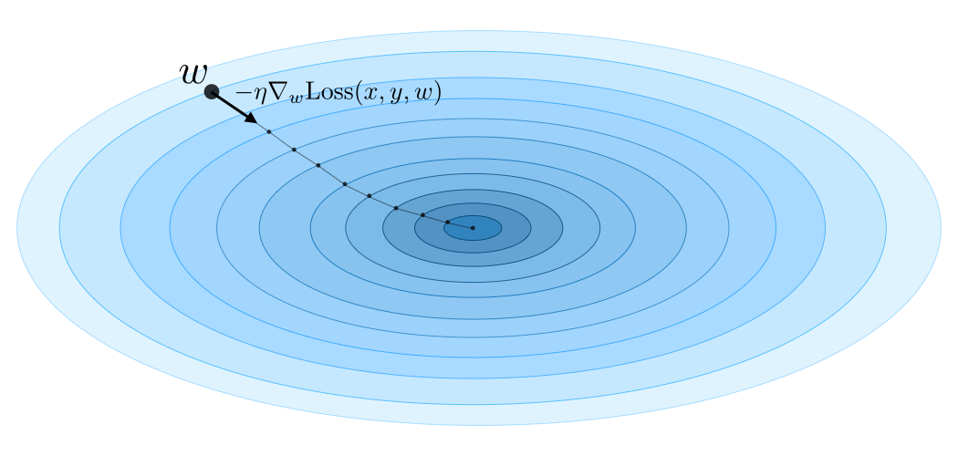
Gradient descent : 梯度下降

$$w\longleftarrow w-\eta\nabla_w \textrm{Loss}(x,y,w)$$

• $\eta \in \mathbb R$
  • learning rate - step size
  • 学习速率 - 每次更新多少

Stochastic gradient descent - SGD : 随机梯度下降 : Stochastic updates - 每次训练更新

Batch gradient descent - BGD : 批量梯度下降 : Batch updates - 一次训练集更新一次

Fine-tuning models

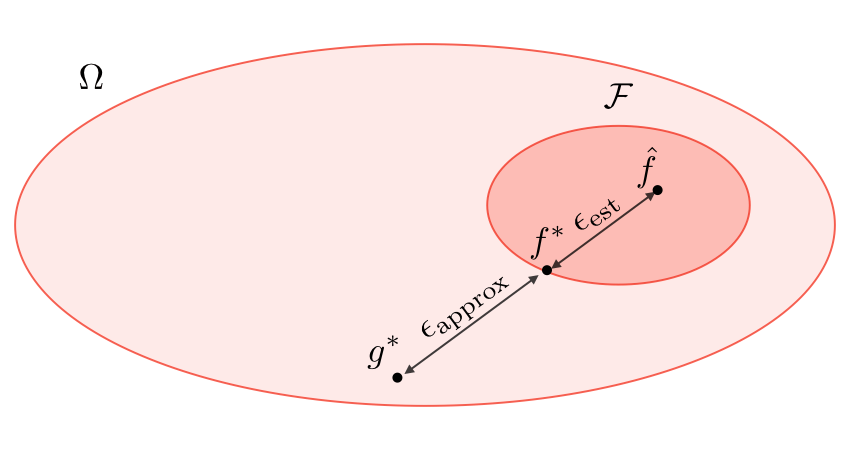
Hypothesis class : 假设类 : $\mathcal{F}=\left\{f_w:w\in\mathbb{R}^d\right\}$

Logistic function : 逻辑函数 : $\sigma$ - sigmoid function

$$\boxed{\forall z\in]-\infty,+\infty[,\quad\sigma(z)=\frac{1}{1+e^{-z}}}$$ $$\sigma'(z)=\sigma(z)(1-\sigma(z))$$

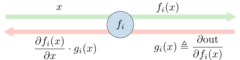
Backpropagation : 后向传播 : $g_i=\frac{\partial\textrm{out}}{\partial f_i}$

Approximation error : hypothesis <-> predictor : $\epsilon_\text{approx}$

Estimation error : predictor <-> best predictor : $\epsilon_\text{est}$

• Regularization
  • keep the model from overfitting
  • LASSO
    • Shrinks coefficients to 0
    • Good for variable selection
  • Ridge
    • Makes coefficients smaller
  • Elastic Net
    • Tradeoff between variable selection and small coefficients
• Hyperparameters
• Sets vocabulary

Unsupervised Learning

k-means

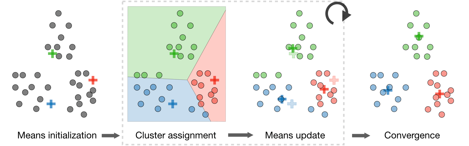
Clustering : $n \in \mathcal D _ \textrm{train}$, clustering 将点 $\phi(x_i)$ 划分为 $k$ 类 $z_i \in \{1,...,k\}$

Objective function : 初始化 clustering 的函数 : 选取 $k$ 个点作为初始的 $k$ 个 cluster 的中心点 : $\textrm{Loss}_{\textrm{k-means}}(x,\mu)=\sum_{i=1}^n||\phi(x*i)-\mu*{z_i}||^2$

k-means : 1. 随机选取 $k$ 个点作为初始的 $k$ 个 cluster 的中心点 - Objective function 2. 计算每个点到 $k$ 个 cluster 的中心点的距离 - Algorithm 3. 将每个点划分到距离最近的 cluster 4. 重新计算每个 cluster 的中心点 5. 重复 2-4 直到收敛

Algorithm

$$\boxed{z*i=\underset{j}{\textrm{arg min}}||\phi(x_i)-\mu_j||^2}\quad\textrm{and}\quad\boxed{\mu_j=\frac{\displaystyle\sum*{i=1}^n1*{\{z_i=j\}}\phi(x_i)}{\displaystyle\sum*{i=1}^n1\_{\{z_i=j\}}}}$$

Principal Component Analysis

• Eigenvalue, eigenvector

$$\boxed{Az=\lambda z}$$

Spectral theorem

$$\exists\Lambda\textrm{ diagonal},\quad A=U\Lambda U^T$$ $$\boxed{\phi*j(x_i)\leftarrow\frac{\phi_j(x_i)-\mu_j}{\sigma_j}}\quad\textrm{where}\quad\boxed{\mu_j = \frac{1}{n}\sum*{i=1}^n\phi*j(x_i)}\quad\textrm{and}\quad\boxed{\sigma_j^2=\frac{1}{n}\sum*{i=1}^n(\phi_j(x_i)-\mu_j)^2}$$

Misc

• $y = w_1x_1 + w_2x_2 + ... + w_nx_n + b$
  • $y$ is the output
  • $x_i$ is the input
  • $w_i$ is the weight
  • $b$ is the bias
• 有监督学习
  • 有输入和输出
  • 输入是特征
  • 输出是标签
  • 通过学习输入和输出的关系, 从而预测未知的输出