CS221 AI: Principles and Techniques
- 基于刺激的模型 - Reflex-based models
- 基于状态的模型 - States-based models
- 基于变量的模型 - variable
- 基于逻辑的模型 - logic
- https://www.youtube.com/watch?v=J8Eh7RqggsU&list=PLoROMvodv4rO1NB9TD4iUZ3qghGEGtqNX
- https://www.youtube.com/watch?v=ZiwogMtbjr4&list=PLoROMvodv4rOca_Ovz1DvdtWuz8BfSWL2
- shervine cs-221
Stanford CS221: Artificial Intelligence: Principles and Techniques | Autumn 2021
Lession 1: Overview
- Reflex-based models
- 基于 反射/刺激 的模型
- 最简单的模型,不考虑历史,只考虑当前情况
- Binary Classification
- 二元分类
- 输出二元结果 - true/false, yes/no, positive/negative, 1/-1, 1/0
- Regression
- 回归
- 输出实数结果
- Structured prediction
- 结构化预测
- 输出复杂对象
Lession 2: Linear Regression
- Linear regression framework
- 线性回归框架
- Decision boundary - 一条线
- Hypothesis class - 假设类 - 哪些预测是可能的
- Loss function - 损失函数 - 如何衡量预测的好坏
- Optimization algorithm - 优化算法 - 如何找到最好的预测
- Decision boundary - 一条线
- Hypothesis class
- 假设类
- 哪些预测是可能的
符号说明
| name | notation | 含义 |
|---|---|---|
| weight vector | 权重向量 | |
| feature extractor | 特征提取器 | |
| feature vector | 特征向量 | |
| train set | 训练集 | |
| test set | 测试集 |
- Feature vector
- 特征向量
- 特征工程 - feature-engineering
- 将原始数据抽象为特征向量
- 特征工程 - feature-engineering
- Score
- 分数
- 如果是最终结果,则代针对某个结论的肯定程度
- 如果是最终结果,则代针对某个结论的肯定程度
- w - weight - 权重
- 对于一个输出,不同的特征对输出的影响不同
- 例如: 一个人的身高,体重,年龄,性别,对于 性别和年龄 的影响不同
- s - score - 分数
- 特征*权重
- 例如: 0.78 是 男性
- Loss function
- 损失函数
- 评价模型的预测值和真实值不一样的程度
- 分为 经验风险损失函数 和 结构风险损失函数
- 评价模型的预测值和真实值不一样的程度
- TrainLoss
- 训练损失
- 在训练中希望减小的值
- value of the objective function that you are minimizing
- 在训练中希望减小的值
机器学习目标
最小化 TrainLoss/训练损失
- gradient
- the gradient is the direction that increases the training loss the most
- 梯度 是让训练损失最大化的方向
- 梯度 是让训练损失最大化的方向
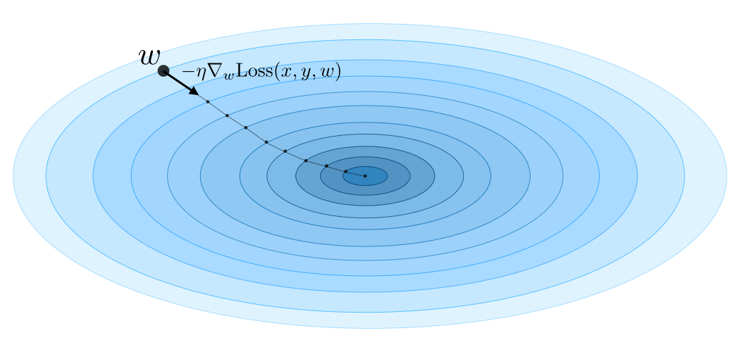
gradient descent - 梯度下降算法
- 初始化
- for
- learning rate - step size
- 学习速率 - 每次更新多少
- 权重 在每个周期被更新 - Machine 学习的内容
- Objective function
- 目标函数
- 统称
- loss function is a part of a cost function which is a type of an objective function.
- Objective function 一般指需要 优化 的函数
- Loss/Cost function 一般指需要 最小化 的函数
- 统称
Note 使用每个 loss 的平均作为初始 TrainLoss
Note
- 的 gradient/ 的转换逻辑后面会讲到
- 使用 squared loss 的 gradient
import Admonition from '@theme/Admonition'; import Tabs from '@theme/Tabs'; import TabItem from '@theme/TabItem'; import {Lession2Demo} from '@theme/CS221';
💡Demo
代码:
function train({ iterations = 200, learningRate = 0.1, log = console.log.bind(console) } = {}) {
  // 训练集
  const trainSet = [
    [1, 1],
    [2, 3],
    [4, 3],
  ];
  log(`train epochs:${iterations} eta:${learningRate}`);
  // Optimization problem
  // 1/3 * sum((w*phi(x) - y) ^ 2)
  const trainLoss = (w) => {
    let sum = 0;
    for (const [x, y] of trainSet) {
      sum += (w[0] * 1 + w[1] * x - y) ** 2;
    }
    return sum * (1 / trainSet.length);
  };
  // 1/3 * sum(2(w*phi(x) - y)phi(x))
  const gradientTrainLoss = (w) => {
    let sum = [0, 0];
    for (const [x, y] of trainSet) {
      let d = 2 * (w[0] * 1 + w[1] * x - y);
      let z = [d * 1, d * x];
      sum = [sum[0] + z[0], sum[1] + z[1]];
    }
    const loss = [sum[0] * (1.0 / trainSet.length), sum[1] * (1.0 / trainSet.length)];
    return loss;
  };
  // Optimization algorithm
  const gradientDescent = (F, gradientF, initialWeightVector) => {
    let w = initialWeightVector;
    let eta = learningRate;
    for (let i = 0; i < iterations; i++) {
      let value = F(w);
      let gradient = gradientF(w);
      w = [w[0] - eta * gradient[0], w[1] - eta * gradient[1]];
      //
      log(`epoch ${i + 1}:`, `w: ${w}, F(w)=${value}, gradient: ${gradient}`);
    }
    return w;
  };
  const w = gradientDescent(trainLoss, gradientTrainLoss, [0, 0]);
  log(`w: ${w}`);
  return { w };
}

向量计算
Lession 3: Linear Classification
- which classfiers are possible - 有哪些可能分类器 - 假设类 - hypothesis class
- how good is a classifier - 评价标准 - 损失函数 - loss function
- how to compute the best classifier - 如何计算 - 优化算法 - optimization algorithm
- Decision boundary
- 决策边界
- for
- Binary classfier
- 二分类器
-
- 输出 label
- Hypothesis class
- 假设类
- score
- 分数
- 可信度 - how confident the classifier is
- margin
- 边距
- 正确度 - how correct the classifier is
- Loss function
- 损失函数

训练目标 梯度下降
- 由于使用了 zero-one loss,此时梯度大多数都是为 0
- 因此无法正常下降,需要使用其他损失函数
- Hinge loss
- 避免 zero-one loss ≤ 0 时大多为 0 的问题
- Logistic loss
- 在超过 1 后还在尝试增加 margin

💡Demo
代码:
TODO
TODO

Lession 4: SGD
Lession 5: Group DRO
Lession 6: Non-Linear Features
Lession 7: Feature Template
Lession 8: Neural Networks
Lession 9: Backpropagation
Lession 10: Differentiable Programming
Lession 11: Generalization
Lession 12: Best Practices
Lession 13: K-means
Misc
- Cost function
- sum of loss × weight
- Mean Squared Error